OpenVDB
![]()
Introduction
Both gases and liquids are fluids. LightWave 2018 introduced us to the importation of existing OpenVDB simulations, Lightwave 2019 presented a robust framework based upon the industry-standard OpenVDB toolset, and LightWave 2020 expands with new tools and workflows. This toolset was developed by DreamWorks Animation, primarily by Ken Museth, Peter Cucka, Mihai Aldén, and David Hill, for use in volumetric applications typically encountered in feature film and expands on this foundation providing backward compatibility with Lightwave’s existing particle simulation tools - ParticleFX and Flocking - while also introducing a new workflow for entirely VDB-based simulations.
In most cases, gases are handled by the OpenVDB Primitive type introduced in 2018 with a dedicated node editor. This provides fog-like raymarched volumetric rendering of thin particles such as smoke and fire.
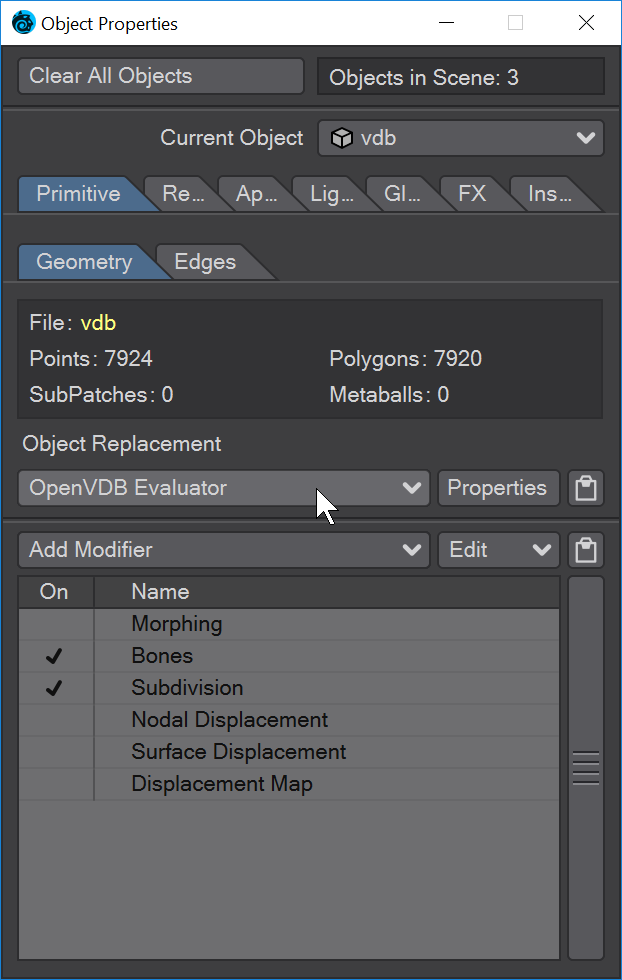
Fluids, on the other hand, will mostly be generated as polygonal surfaces - called Iso Surfaces - using the OpenVDB Evaluator found in the Object Properties Object Replacement dropdown menu.
The key element in OpenVDB is the grid, more precisely "the efficient storage and manipulation of sparse volumetric data discretized on three-dimensional grids." Think of grids as an object’s bounding box that can be subdivided into smaller cells where something exists (such as a surface, points, particles…) while ignoring the empty cells, hence the "sparse" part of the description.
These cells are Voxels and act much like pixels in an image, but representing 3D volumetric shapes. The smaller the voxel size, the more detailed the object will be.
The beauty behind this system is that it entirely ignores empty cells decreasing memory and disk usage while making the rendering of volumes much faster.
This new feature gives the user the power to create volumes from meshes and meshes from volumes
OpenVDB Evaluator
To create your own OpenVDB object, you need to start with a source object and a null with the OpenVDB Evaluator Object Replacement added. OpenVDB objects can be made from meshes, primitives and even other volumetrics.
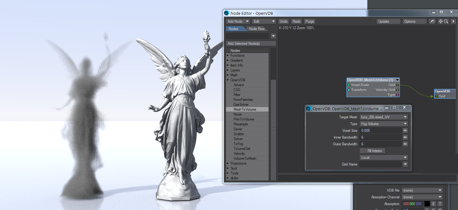
![]() Once you have your target mesh and null to direct it to, open the node editor by clicking on the Properties button next to the OpenVDB Evaluator entry. The destination node:
Once you have your target mesh and null to direct it to, open the node editor by clicking on the Properties button next to the OpenVDB Evaluator entry. The destination node:
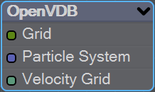
contains three entries. A scalar-based grid input, an OpenVDB-specific Particle System input, and a vector-based velocity grid input. The scalar grid is the one you'll use most often for fixed shapes. The new Particle System input gives you the ability to output a particle system from the OpenVDB Evaluator for further work downstream. If motion blur is enabled and there is a velocity grid, a deformer will be added to the object modifiers list allowing for subframe evaluation of the grid using the velocity input.
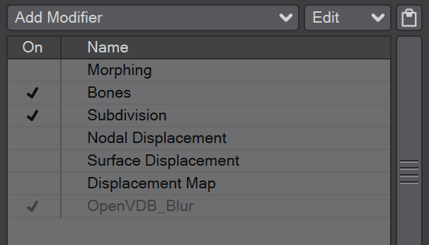
The OpenVDB Blur deformer cannot be interacted with by the user. It has no UI, cannot be added or deleted except automatically by Layout
Double-clicking on the destination node will open its settings window
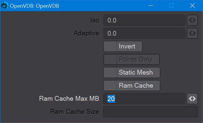
- Iso - The iso value is considered to be the zero-crossing of the grid's field of values. This zero-crossing is where polygons are constructed
- Adaptive - Values above zero will consolidate small voxel size polygons into larger polygons as flatness allows
- Invert - Fog volumes can be input, but due to the representational difference between them (unsigned ) and SDF (signed) volumes, the polygons appear backward. Checking Invert will flip the polygons for that case. Additionally, you will need to move the Iso surface above 0
- Points Only - Useful for outputting a particle system still as particles for use with other systems in Layout, like Flocking, Instancing, HyperVoxels, etc.
- Static Mesh - Stops frame-based re-evaluation of a resulting OpenVDB mesh
- RAM Cache - Caches the Grid input to RAM, up to the Max MB setting. If the cache exceeds this amount caching is released, starting with the frame furthest from the current frame
- RAM Cache Max MB - The total RAM cache for the scene
- RAM Cache Size - This field should show the current size of the RAM cache, and currently doesn't. The error will be corrected.
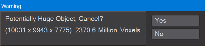
Layout will provide you with a warning message if you create a vast number of voxels.
Common
OpenVDB nodes may have the following common settings:
- Voxel Size - Size of the voxel grid in meters (LightWave supports uniform grids); the size of the voxel "blocks" that will make up your object
- Inner Bandwidth - Inner Bandwidth for level set in voxels
- Outer Bandwidth - Outer Bandwidth for level set in voxels. For fog volumes, this defines the "softness" until maximum density is reached.
- Fill Interior - Toggle for whether the volume will be solid when cut into or just a shell - like polygons are. Turning on Fill Interior with a Fog Volume will soften the outside of the fog
- Coordinate System - How the voxel will be transformed. There are three choices
- Local - No transform
- World - Transform into world space
- Parent - Use the parent item's space
- Grid Name - the base name of
savedgrid.vdbfiles. Files will be appended with the frame number and written with temperature, density, and velocity grids
Solid Volumes from Meshes and other Scene Items
Creating volumes from meshes relies on polygons being tris or quads. NGons are not supported
Creating a volume this way requires a target mesh, primitive shape or Particle emitter that needs to be in the scene. It can be out of camera view, hidden from render and hidden in OpenGL and the Object Replacement will still work. To create a volume from this item requires adding a null and using the Object Replacement entry OpenVDB Evaluator. Clicking Properties for it will bring up a Node Editor window.
 Mesh To Volume
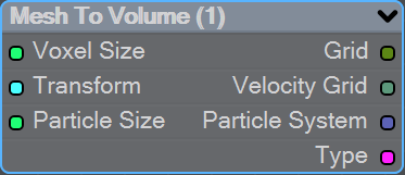
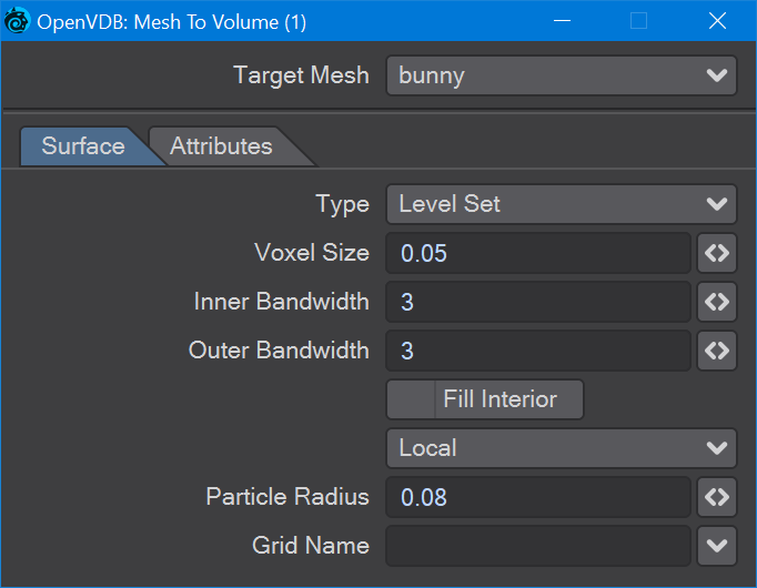
In the OpenVDB nodes group, Mesh To Volume will be the node to convert your mesh objects into volumes. There are two choices for conversion, Fog Volume will convert a mesh into a volumetric fog, much like the image at the top of this page, but you need to use an OpenVDB primitive. The second option is Level Set, which creates a volumetric mesh object. The Voxel Size setting will determine the resolution of your volumetric object. For the Logo Rezzing Up example, a Scalar Constant node was used with an envelope that went from the default 1 down to 0.0025 to create the increasing resolution of the volume.
Particle Radius is where you set the size of individual particles if you will be outputting a particle system from this node.
The new Attributes tab, added in 2020, is where you can transfer details like vertex maps or surfacing information from the original mesh to your OpenVDB object.

Surfaces will all be added. You cannot just choose one.
Shape To Volume
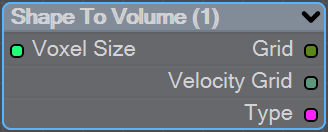
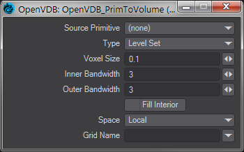
Will create a volume from LightWave primitive objects.
Fog To LevelSet
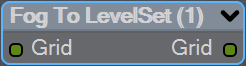
Converts a Fog grid to a Level Set mesh object. A fog grid can be imported using the OpenVDB Info node. Double-clicking the node brings up its window with Iso setting and Normalize toggle.
 From Particles
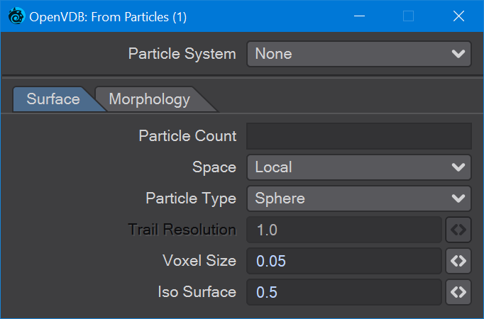
New to 2020. There is now a Particle System output to send particles directly to the Editor Input. You can choose to represent particles as individual spheres or a trail (of connected spheres). When you select Trail, a Trail Resolution setting becomes available. Higher values mean more trail particles and might be needed for high-velocity trails.

The Morphology tab includes elements that are found in the Filter node that can be applied directly, without needing a discrete Filter node.
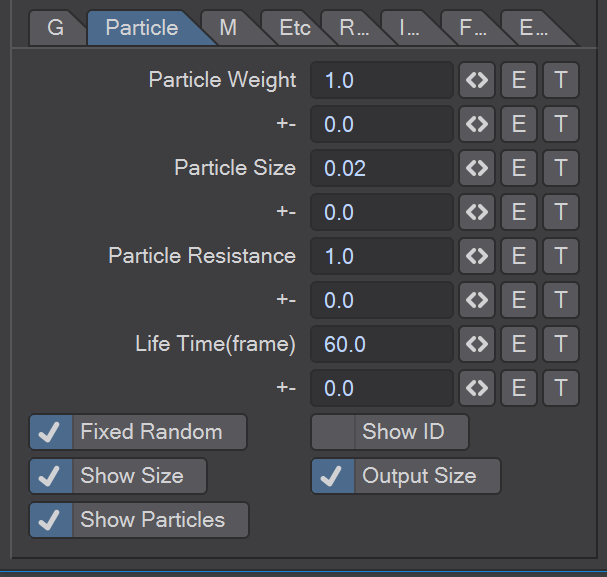
When you have a particle emitter being meshed, you cannot bring up the particle properties, as upon meshing (the OpenVDB Evaluator being an object replacement procedure), the PFX Emitter server pane will close. The only way to adjust particle properties, in this case, is by using the modal FX Browser panel.
The same is true for other server pane items - changing the subdivision level, for example - but in that case, the only workaround is to disable the VDB object in the Scene Editor by unchecking the render flag.
FX Emitter particles must have a Size, and that size must be output with the Output Size toggle. You don't need to Show Size; it just helps visually.
This node will create a volumetric object from a stream of particles created using the FX Emitter or the Scatter or Solver nodes here. You have the option to either create sphere shapes or a trail per particle derived from their position, radius, and velocity. Each trail is generated as CSG unions of sphere instances with a decreasing radius.
The direction of a trail is inverse to the direction of the Velocity vector, with a length of |V|. The radius at the head of the trail is given by the radius of the particle and the radius at the tail of the trail is Rmin voxel units which has a default value of 1.5 corresponding to the Nyquist frequency.
- Particle System - A dropdown for choosing the specific particle system you want to use. Using the Input ghosts this control
There are two tabs next: - Surface - Details how the particles look:
- Particle Count - A readout of attached particle system particle count
- Space - Choose whether your particles are situated in Local, Parent or World Space
- Particle Type - Choice between Sphere and Trail. Sphere will create distinct bubbles whereas Trail will attempt to use particle velocity to create a trail of diminishing size. Each trail is generated as CSG unions of sphere instances with a decreasing radius
- Trail Resolution - Only available when the Trail Particle Type is chosen. The default of 1.0 trails off "normally". Less than 1.0 means fewer trail particles and separation might be noticeable. More than 1.0 means more trail particles are created. Higher trail speeds might need more particles to stay stream-like so separation doesn't show
- Voxel Size - Size of the Voxel for the particles. Voxels sizes in a network should be the same, especially combining or collisions between VDB grids
- Iso Surface - Iso sizes in a network can be different but the editor input node will create the final meshing
- Morphology - Operators so additional nodes are not needed
- Dilation - Dilate the grid along its normals making it bigger
- Closing - Dilate the grid to close holes then erode closing openings
- Smoothing - Gaussian smoothing
Gaseous Volumes from Scene items
Gas Solver
Gas solver. Use Stam's stable fluids method to advect density and temperatures. Both the density and the temperature affect the fluid’s velocity. Heavy smoke tends to fall downwards due to gravity while hot gases tend to rise due to buoyancy. We use a simple model to account for these effects by defining external forces that are directly proportional to the density and the temperature.
buoyancy = (-densityscale * density * Vec3f(0, 1, 0)) + (temperaturescale * temperature * Vec3f(0, 1, 0));
External forces can be added on the Force Grid input. This input accounts for external forces like gravity, wind, turbulence and merely is added onto the end of the momentum equation.
Temperature Tab
- Ambient Temperature - Ambient air temperature
- Clamp Temperature - Clamps the temperature to the minimum value set below (otherwise the gas cools to the point where it falls like dry ice)
- Min - The minimum temperature (in Celsius) for the gas to fall to
- Normalize Temperature Grid - Outputs the temperature grid as a scale between 0 and 1, rather than, say, 60 and 900
- Fuel Temperature - Fuel temperature as it is emitted
- Gas Density - Density of emitted smoke from the fuel grid
- Fuel Velocity - Velocity of emitted smoke and heat from the fuel grid
- Density Scale - Scale of the downward pull on dense smoke
- Buoyancy Scale - Scale of the temperature gradient pulling smoke upward
- Cooling Scale - Scales the cooling rate
- Dissipation - The amount of density that falls off over each iteration so that the gas thins over time
Advection Tab
- Spacial - Set the spatial finite difference scheme. In other words, how accurately the gradients of the signed distance field are computed depends on your pick of interpolator. The choices further through the list are more accurate but take more time
- Spacial Tracker - Set the spatial finite difference scheme. How accurately time is evolved within the timestep. The choices further through the list are more accurate but take more time
- Temporal - Set the temporal integration scheme. How accurately time is evolved within the renormalization stage. The choices further through the list are more accurate but take more time
- Temporal Tracker - Set the temporal integration scheme. How accurately time is evolved within the timestep. The choices further through the list are more accurate but take more time
- Integrator - Set the numerical advection scheme. The choices further through the list are more accurate but take more time
- Limiter - Set the limiter scheme used to stabilize the second-order MacCormack and BFECC schemes
- Max Divergence Steps - Maximum number of iterations of the pressure solver
- Advection Sub Steps - Substeps per integration step. The only reason to increase it above its default value of one is to reduce the memory footprint from dilations - likely at the cost of more smoothing!
- Curl Scale - Curl strength of the vorticity confinement
Domain Tab
- Boundary - One of three choices:
- Free Slip - Velocity is negated at the boundary axis
- No Slip - Velocity is set to 0 at the boundary
- Outflow - The grid is clipped at the boundary
The Min and Max domain fields are for setting the minimum and maximum extents (corners) of the simulation's domain.
Cache Tab
- Cache Grids - Toggle for enabling the caching of grids to Cache Path folder. Once cached they can be loaded without simulation
- Cache Name - Base name of saved grid . vdb files. Files will be appended with the frame number. Files will be written with temperature, density, and velocity grids
- Grid Path - Path to save folder
- Clear Cache - Clear all files in the cache folder
- Behavior - A dropdown with three choices:
- Manual - Cache control is completely up to the user
- Warn - A message will warn "The cache is invalid, should it be cleared?"
- Automatic - The cache is cleared automatically, when necessary
To Fog Volume
Converts an SDF grid (signed) to a fog volume (unsigned) with a filled interior. There are no options.
Tools
You can manipulate OpenVDB volumes with the following included tools.
Advect
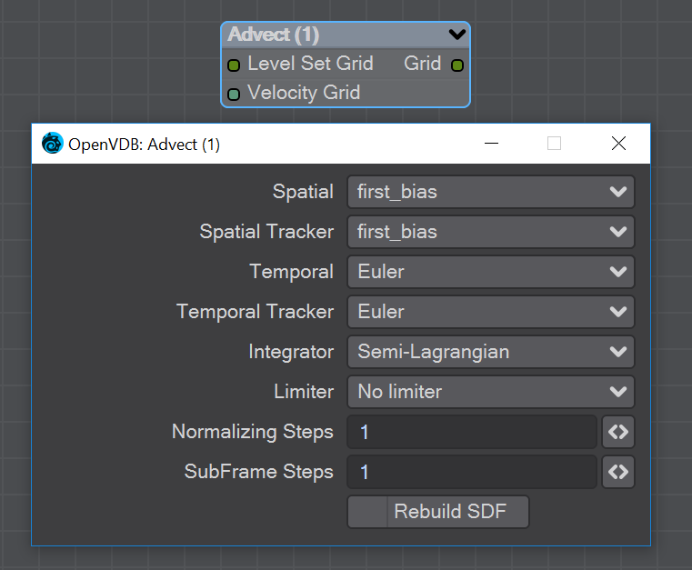
Advect a Signed SDF grid with a velocity grid. Requires a Velocity Grid vector to give movement and direction.
- Spatial - Set the spatial finite difference scheme. In other words, how accurately the gradients of the signed distance field are computed depends on your pick of interpolator. The choices further through the list are more accurate but take more time
- Spatial Tracker - Set the spatial finite difference scheme. How accurately time is evolved within the timestep. The choices further through the list are more accurate but take more time
- Temporal - Set the temporal integration scheme. How accurately time is evolved within the renormalization stage. The choices further through the list are more accurate but take more time
- Temporal Tracker - Set the temporal integration scheme. How accurately time is evolved within the timestep. The choices further through the list are more accurate but take more time
- Integrator - Set the numerical advection scheme. The choices further through the list are more accurate but take more time
- Limiter - Set the limiter scheme used to stabilize the second-order MacCormack and BFECC schemes
- Normalizing Steps - A number of renormalization passes can be performed between each substep to convert it back into a proper signed distance field. Prevents jerky motion but soften and slows the velocities
- SubFrame Steps - Substeps per integration step. The only reason to increase it above its default value of one is to reduce the memory footprint from dilations - likely at the cost of more smoothing!
- Rebuild SDF - Toggle to rebuild and retrack the narrow band of the SDF
Advect Points
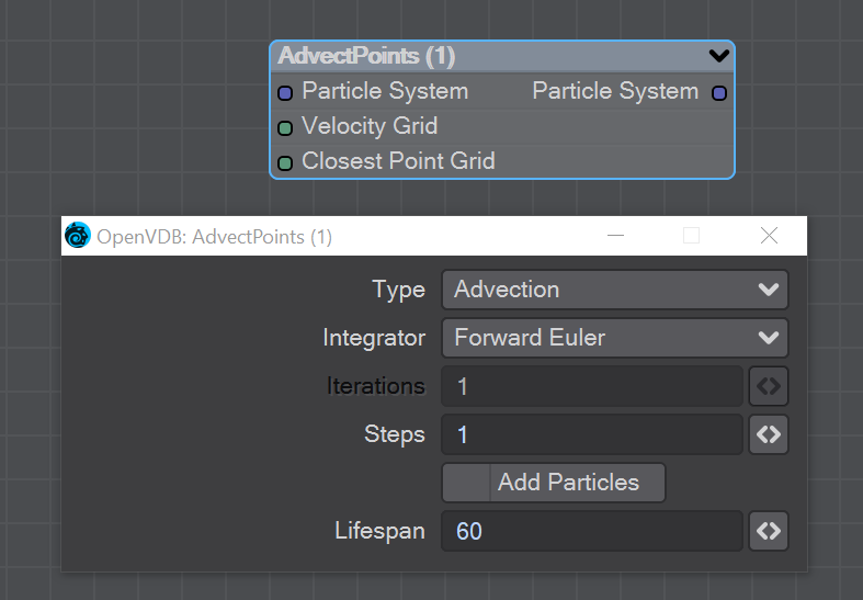
This node will advect the points in a particle system along a velocity field. The first thing you need is a particle system to use. Node inputs are:
- Particle System - Particle system to advect
- Velocity Grid - This must be a vector-valued VDB primitive. You can use the Vector Merge node to turn a vel.[xyz] triple into a single primitive
- Closest Point Grid - Used for projection and constrained advection
In the node's panel, the controls are as follows:
- Type - Three types are proposed:
- Advection - Move the point along the velocity field
- Projection - Move the point to the nearest surface point
- Constrained Advection - Move the along the velocity field, and then project using the closest point field. This forces the particles to remain on a surface
- Integration - Later options in the list are slower but better at following the velocity field
- Iterations - Number of times to try projecting to the nearest point on the surface. Projecting might not move exactly to the surface on the first try. More iterations are slower but give a more accurate projection
- Steps - How many times to repeat the advection step This will produce a more accurate motion, especially if large time steps or high velocities are present
- Add Particles - At each frame add the input particles to the advection
- Lifespan - How many frames the advected points will live for
Analysis
This node presents various grid manipulations. Depending on the input grid type and the operation the output grid type will vary. Once an input is connected and the grid type is known the list of available operations will be collapsed to only show appropriate choices. Finally, if you change the operation the grid output will disconnect (ie scalar to vector).
- Gradient - Vector that points perpendicular to the values basically un-normalized normals (Scalar - Vector)
- Curvature - A measure of the surface curvature (Scalar - Scalar)
- Laplacian - A smoothed version of the input (Scalar - Scalar)
- Closest Point Transform - Direction to the closest point (Scalar - Vector)
- Divergence - A measure of the change in quantities (Vector - Scalar)
- Curl - A direction perpendicular to the input grid vectors (Vector - Vector)
- Magnitude - The scale of the input vectors (Vector - Scalar)
- Normalize - Normalized input vectors (Vector - Vector)
There is also a Scale input for further adjustment.
CSG
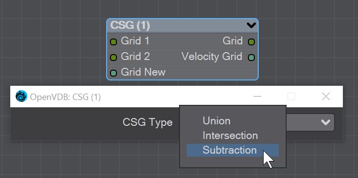
Takes the Result from two SDF shapes and combines them in the fashion that should be familiar by now -
- Union - Combines the two shapes, and is the default option
- Intersection - Only leaves the parts of the two shapes that overlap
- Subtraction - Removes Shape A from Shape B
The velocity of the input grids will be reconstructed and output.
Combine
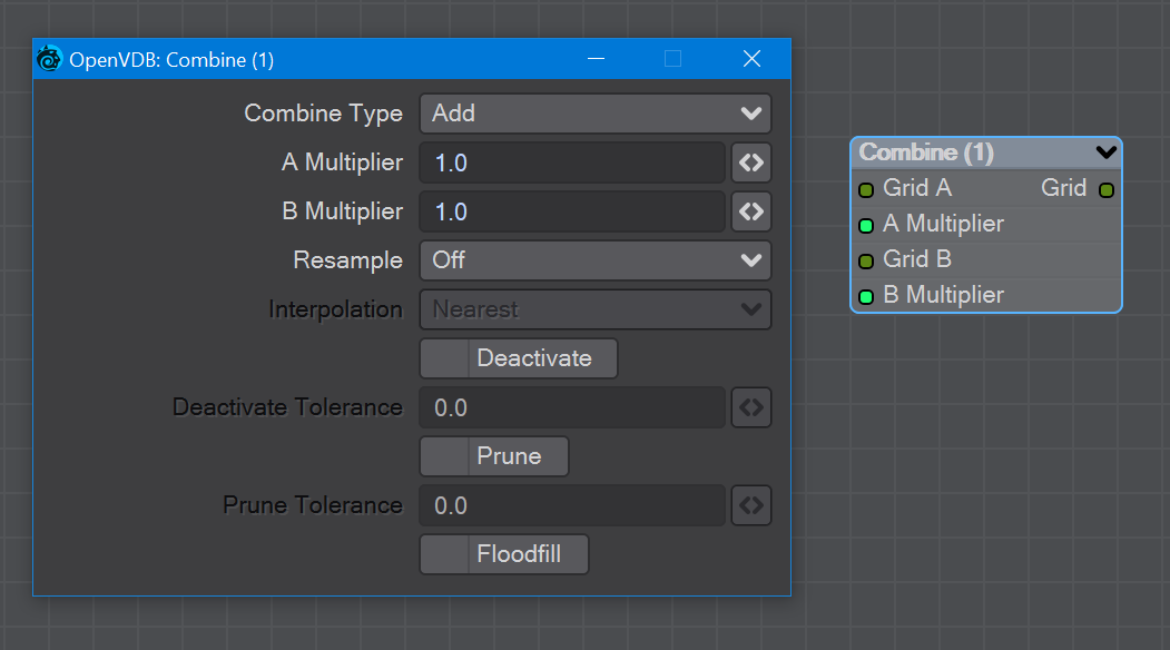
Combines grids using scalar operations.
- Combination type - The different math operators that can be brought to bear:
- Copy A - Use A , ignore B
- Copy B - Use B, ignore A
- Invert - Use 1 minus A
- Add - Add the values of A and B (Using Add for fog volumes, which have density values between 0 and 1, will push densities over 1 and cause a bright interface between the input volumes when rendered. To avoid this problem, try using the Blend 2 option)
- Subtract - Subtract the values of B from the values of A
- Multiply - Multiply the values of A and B
- Divide - Divide the values of A by B
- Maximum - Use the maximum of each corresponding value from A and B (Using this for fog volumes, which have density values between 0 and 1, can produce a dark interface between the inputs when rendered, due to the binary nature of choosing a value from either from A or B. To avoid this problem use Blend 1 instead)
- Minimum - Use the minimum of each corresponding value from A and B
- Blend 1 - (1 - A) * B. This is similar to SDF Difference, except for fog volumes, and can also be viewed as a "soft cutout" operation It is typically used to clear out an area around characters in a dust simulation or some other environmental volume
- Blend 2 - A + (1 - A) * B. This is similar to SDF Union, except for fog volumes, and can also be viewed as a "soft union" or "merge" operation. Consider using this over the Maximum or Add operations for fog volumes
- A Multiplier - Multiply voxel values in the A VDB by a scalar before combining the A VDB with the B VDB
- B Multiplier - Multiply voxel values in the B VDB by a scalar before combining the A VDB with the B VDB
- Resample - Multiple options here. If the A and B VDBs have different transforms, one VDB should be resampled to match the other before the two are combined. Also, level set VDBs should have matching background values (i.e., matching narrow band widths):
- Off - No resampling
- B to Match A - Resample B so that the narrow band width is the same as A
- A to Match B - Resample A so that the narrow band width is the same as B
- Higher-res to Match Lower-res - Resample the higher resolution data so that the resolutions match
- Lower-res to Match Higher-res - Resample the lower resolution data so that the resolutions match
- Interpolation - When you choose a resampling option other than Off, the Interpolation choices become available. There are three to choose between:
- Nearest - Nearest Neighbor interpolation is fast but can introduce noticeable sampling artifacts
- Linear - Linear is the middle ground of speed and quality
- Quadratic - Quadratic interpolation is slow but high-quality
- Deactivate - Toggle to deactivate active output voxels whose values equal the output VDB's background value. When this option is checked, the field below becomes active:
- Deactivate Tolerance - When deactivation of background voxels is enabled, voxel values are considered equal to the background if they differ by less than this tolerance
- Deactivate Tolerance - When deactivation of background voxels is enabled, voxel values are considered equal to the background if they differ by less than this tolerance
Prune - Reduce the memory footprint of output VDBs that have (sufficiently large) regions of voxels with the same value
Pruning affects only the memory usage of a VDB. It does not remove voxels, apart from inactive voxels whose value is equal to the background
- Prune Tolerance - When pruning is enabled, voxel values are considered equal if they differ by less than the specified tolerance
- Prune Tolerance - When pruning is enabled, voxel values are considered equal if they differ by less than the specified tolerance
- Flood Fill - Reclassify inactive voxels of level set VDBs as either inside or outside. This option will test inactive voxels to determine if they are inside or outside of an SDF and hence whether they should have negative or positive sign
Filter
![]()
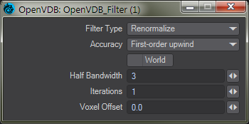

This node adjusts the inner bandwidth of a volumetric signed distance field represented by a VDB volume
Filters the level set grid:
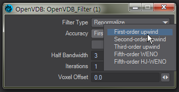
- Filter Type:
- Renormalize - Repair level sets represented by VDB volumes. Certain operations on a level set volume can cause the signed distances to its zero crossing to become invalid. This node iteratively adjusts voxel values to restore proper distance
- Mean Value - This performs the equivalent of a simple box blur by taking the mean of the surrounding values
- Median Value - This chooses the median of the surrounding values, good for homogenizing noisy data to avoid spikes
- Mean Curvature - Finds the average curvature for a location and moves the surface along its normal to smooth out bumps
- Laplacian Flow - Uses a local Laplacian value for movement along a normal
- Dilate - Dilate the grid along its normals making it bigger
- Erode - Erode the grid along its normals making it smaller
- Close - Dilate the grid to close holes then erode closing openings
- Open - Erode the grid then dilate to create openings
- Track - the grid topology is updated by rebuilding the inner band so that it tracks the new iso interface
- Gaussian - Gaussian smoothing
- Resize - Change the width of the inner band of a VDB signed distance field
- Accuracy - Increasingly complex algorithms for the accuracy of the integration
- World - Performs the math for creating the levelset in World space, rather than Local
- Half Bandwidth - Level sets are normally symmetrical on the inner band. Half Bandwidth uses this fact to halve calculation times but at the cost of accuracy
- Iterations - the maximum number of attempts to achieve a divergence-free pressure matrix
- Voxel Offset - Offsets the iso surface from the actual value. For instance, using
Level Set Morph
You will need to freeze subpatched objects as they are not seen by OpenVDB
In a scene, have two polygonal objects and a null. The point and polygon counts don't have to match, or even be close. In the example above, we are going from the Utah teapot with 1,506 polygons, to the Stanford bunny object with roughly 70,000. Use the Object Replacement > OpenVDB Evaluator entry to convert the two objects to OpenVDB (make sure that their Voxel Size fields match) Level Sets. Pipe the Grid outputs from these nodes into the new Level Set Morph node and from that into the destination Grid node.
Morphing between objects involves the nodes we've already outlined. Morphing from one surface into another requires the two surfaces to be changed as well. To do so, in the Surface Editor, pick your morphing null and edit its surface. Double click on the surface name to open the node editor and add:
- Material Tools > Material Mixer
- The surface for one object
- The surface for the other object
- Info > Time

The above node tree will synchronize your surface morphing at the same time as the geometry

The first four controls (Spatial, Spatial Normalize, Temporal, and Temporal Normalize) are graded in terms of rapidity and quality. Change up from the first only if it is posing problems with how the Morph is playing out.
- Normalizing Steps - After morphing the signed distance field, it will often no longer contain valid distances. A number of renormalization passes can be performed to convert it back into a proper signed distance field
- Speed - A scalar to determine how fast your morph occurs
- Invert Alpha Mask - If you have hooked up a grid as an alpha mask, this option allows you to reverse what is alpha'ed out
Noise
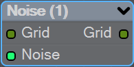
Add the Bump output from an image or a 3D Texture to this node and pipe the output through.
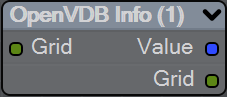
OpenVDB Info
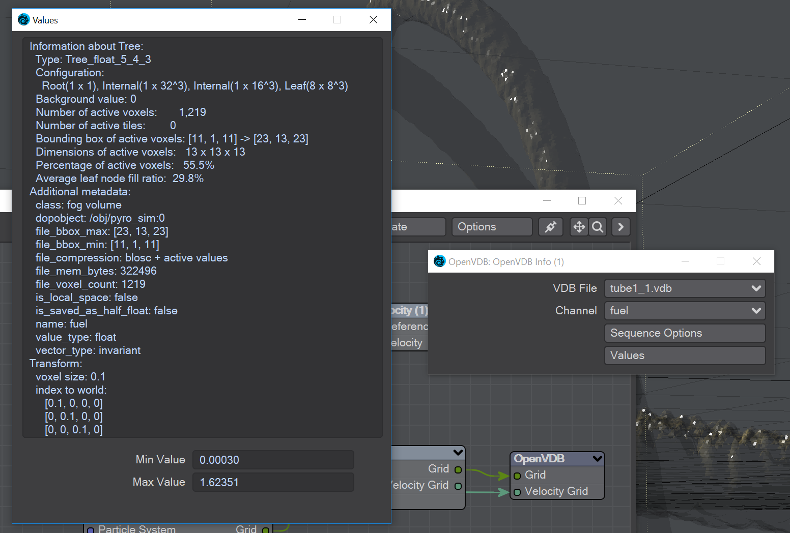
The values for the Fuel channel of a VDB sequence
You can pipe a Level Set or Fog grid into this node and see the values contained within the file, but this node becomes more useful when you load a vdb file directly in the node. You can see info from whatever channels the vdb file contains.
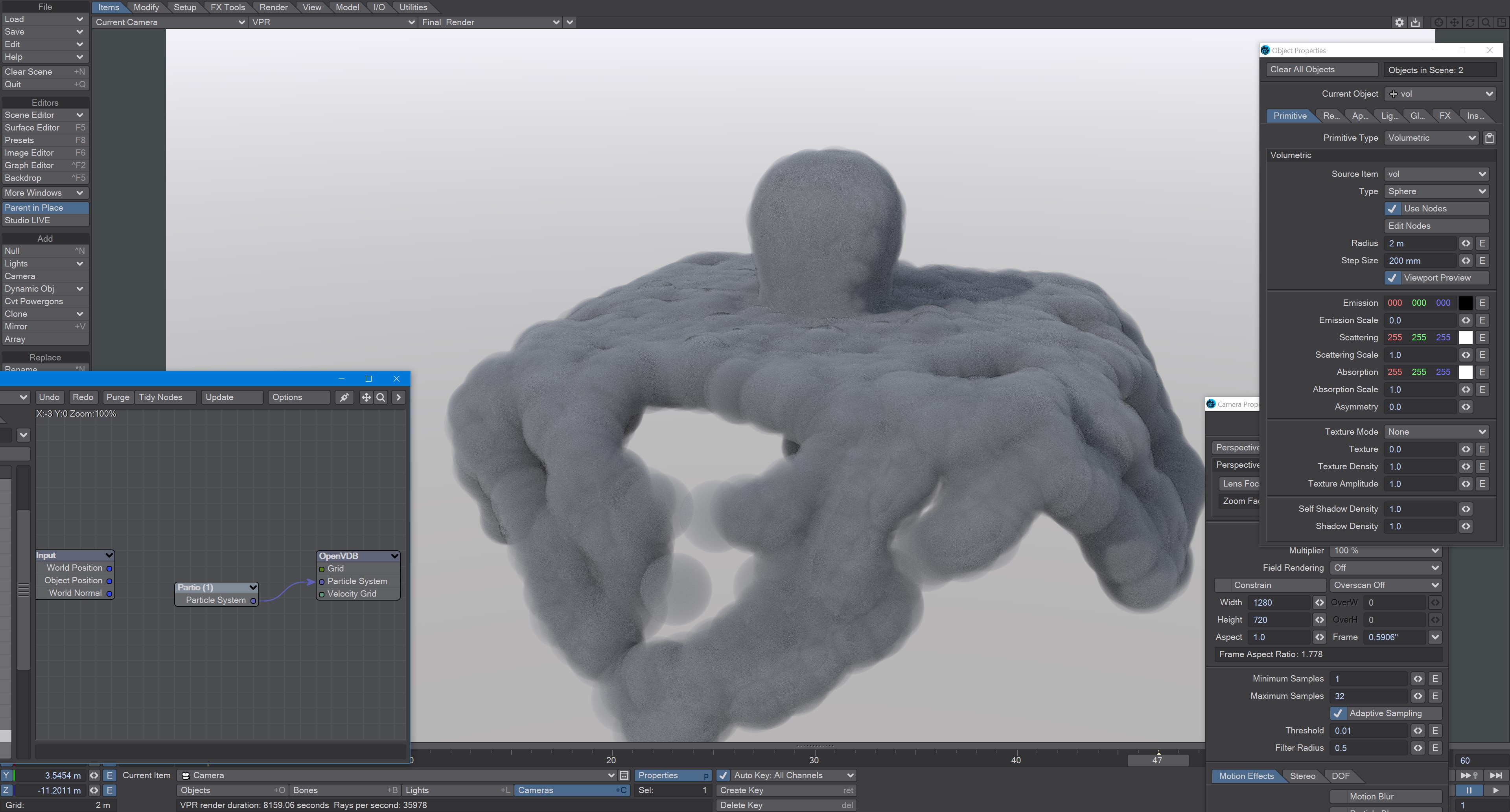
Partio Node
The Partio node is simple in that it has one output and no inputs. Double-clicking on the node shows more depth:
Load Path - Where your particles are located.
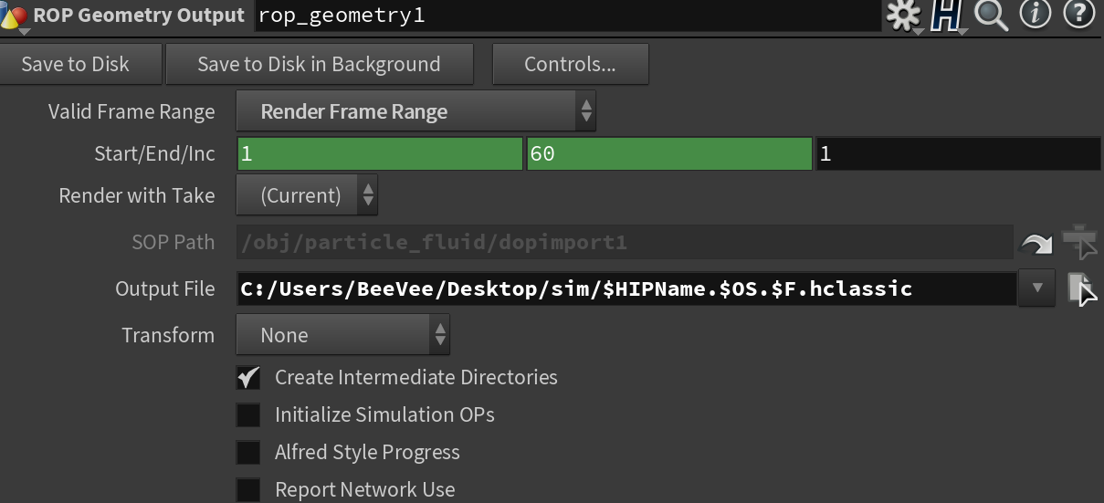
You should place Houdini files in your content directory's GridCache folder to ensure they can be seen by Package Scene.
Target - If you are using a volumetric object with the particle system, make sure it is targeted here
Start Frame - The frame on which to start the simulation in LightWave
Missing Frames - I have Hold (keep the previous frame's contents?) and Blank (leave a gap?)
Size - The particle size. If using a grid, it should be 1.5 times the voxel size or risk being missed
Attributes list
Using the Houdini "vocabulary" here. If you have particles from a different source, the names may be different. The fields are fairly self-explanatory with name, type, and depth. A Float 3 is three scalars, a color for instance. A Float 1 is a simple scalar.
- position - The particle position
- Cd - The diffuse color of the particle
- v - Particle velocity. Can be used as a color or for post blurring, for example
- pscale - The size of the particle
The Partio node has a single output - Particle System. To see these outputs, add an Additional > ParticleInfo node.

Because the outputs are dynamically created, if you are not seeing the outputs you expect, make sure that:
- The ParticleInfo node is addressing the right object (double click the node to check the target)
- The frame you are on actually has particles. It's not before or after the particles appear
- You try stepping the frame forward and back to refresh the node, or moving the ParticleInfo node itself
Once you have exported a stream of HClassic files, you can import them into LightWave using the Partio node. To do so, add a null to an empty scene. Make the null an OpenVDB Evaluator using the Object Replacement dropdown menu. Hit the P button to edit the Evaluator's nodes. Add the Partio node, but you won't see anything until you have chosen from the following
- From Particles - Size in the Partio node should be about 1.5 times the Voxel Size in the From Particles node, sometimes a little bigger. This makes sure the particle spans the voxel cube; smaller and you might not see the particle rasterized.

Using the Partio node with a From Particles node - As Particles - You can go straight from the Partio node to the OpenVDB destination node, turn on particles in the destination node and then just get particles that can be used for other purposes - such as with old-fashioned HyperVoxels.

Don't forget to turn on 'Use Legacy Volumetrics' In the Render Properties > Volumetrics tab
You can also use LightWave's own Volumetric objects. Add another null called "vol". Set the vol null Primitive Type to Volumetric. Use an OpenVDB Evaluator Object Replacement in the Partio's Object Properties window. In the Node Editor, add a Partio node and bring in your Houdini HClassic files. Set the Partio node Target to the vol null.

Hook the Partio node directly to the Destination OpenVDB node. This will output a particle system. Add a new null labeled "vol" and make it a Volumetric object. Set the source item here to vol.
Resample
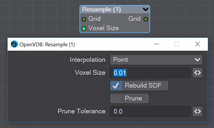
Resample input grid to new voxelsize to output grid.
- Interpolation - Different interpolators with increasing complexity
- Rebuild SDF - Rebuilds and normalizes the narrow band of the level set
- Prune - Removes values from the level set that are smaller than the Prune Tolerance set below
Saver
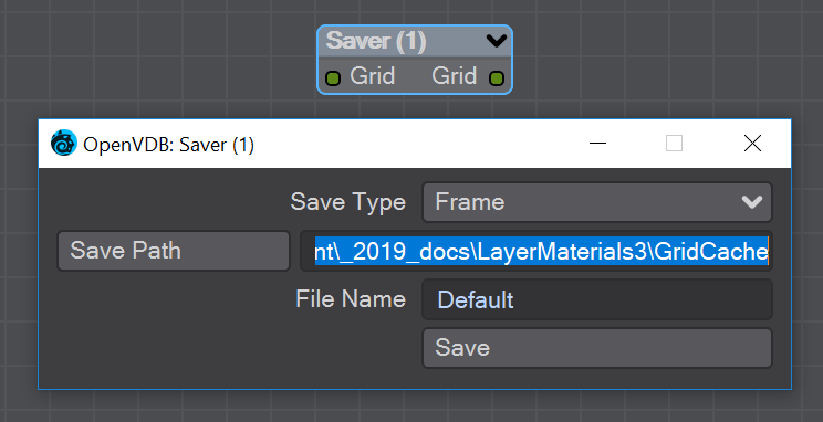
Pipe a grid into here and the frame or sequence is saved as VDB files upon clicking the Save button.
- Save Type - a choice of Frame or Sequence. In both cases, a files or files will be saved using the File Name chosen appended with the frame number
- Save Path - Choose a folder for the frame or sequence
- File Name - The chosen prefix for the frame or sequence
- Save - Immediately saves the frame or sequence. There is no visual confirmation apart from the playhead stepping through the scene in case of a sequence save
To load files saved this way, use the OpenVDB Info node to choose the VDB file and its channel saved.
Scatter
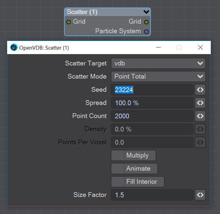
Scatter creates particles on the input grid. The particle system constructed belongs to the scatter target item. Particles can be scattered on or in both SDF and fog volumes.
- Scatter Target - The input grid to scatter on
- Scatter Mode - Dropdown to specify how the particles will be placed:
- Point total - Absolute number of particles to be scattered
- Point Density - Percentage of voxels in which to place a particle
- Points Per Voxel - Number of particles to put in each voxel
- Seed - Sets the random seed
- Spread - Distance to randomly move from the voxel center
Depending on the scatter mode chosen:
- Point Count - When Point Total is chosen (integer)
- Density - When Point Density is picked (percentage)
- Points Per Voxel - When Points per Voxel is chosen (scalar)
- Multiply - Density multiplier
- Animate - Reseed the random generator each frame
- Fill Interior - Fill particles inside the sdf narrow band
- Size Factor - The size of the particles created
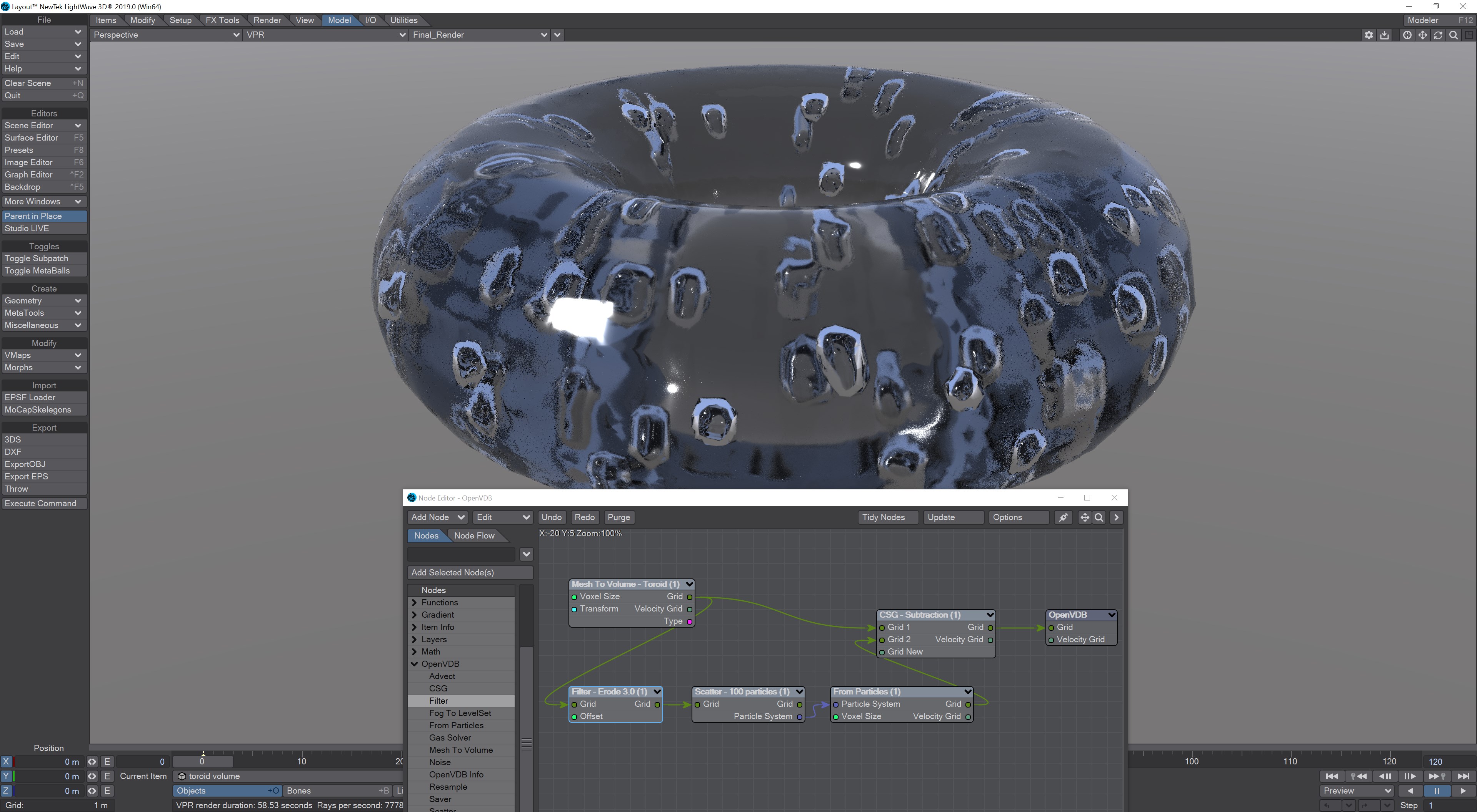
Creating bubbles inside a VDB toroid is simple with the Scatter node. The Filter node has been used here in Erode mode to ensure that the bubbles are created inside the toroid volume and not at the boundary.
Solver
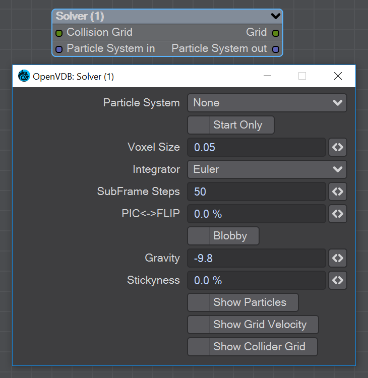
A particle solver that uses a particle system to initialize a temporal PIC/FLIP feedback loop. Particles from the particle system are input as they are born. Then are advected by the integrator using the gravity over the frame substeps. PIC (Particle In Cell) produces smoother motions, and FLIP (FLuid Implicit Particles) is splashier. The two methods can be combined.
The Navier-Stokes equations that the PIC/FLIP system uses do not dictate position but velocity. The vectors contained are not coordinates but velocities. PIC / FLIP is an advection equation, which is how the particles in these objects move within velocity fields.
Particles In Cells (PIC) works by evaluating particles as groups of particles in cells (like voxels)
FLIP stands for FLuid-Implicit Particles and uses a grid rather than particles. Grid-based methods were great for large ocean effects, but not fine detail close up visual effects work. Things can look globby and unrealistic at a small scale (thin fluids).
Inputs
- Collision Grid - SDF grid to be used for collisions
- Particle System input - Use a separate particle system
Outputs
- Grid - Outputs an SDF grid
- Particle System Out - Particle system output
- Start Only - Only uses the first frame of the particle system
- Voxel Size - Size of the gid voxels
- Integrator - In short, the upper choices from this dropdown menu are faster but the lower choices are better quality
- Subframe Steps - More steps per frame is more accurate but takes longer
- PIC↔FLIP - Ratio of PIC velocities to FLIP velocities
- Blobby - Check to treat the particles as spheres
- Gravity - Downward pull in meters per second squared
- Stickiness - Amount of velocity absorbed by contact with collision object
- The next three checkmarks are to help visualize the grid:
- Show Particles
- Show Grid velocity
- Show Collider grid
The Solver is time-based so scrubbing the scene will break it, particularly going backward. Create previews to see a smooth animation if your scene is too heavy.
Vector Merge and Split
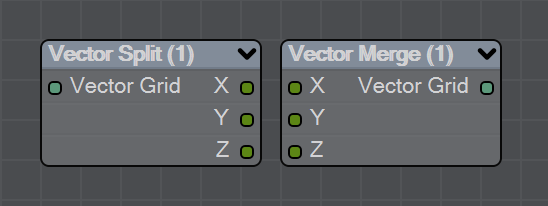
New to LightWave 2020 is a pair of nodes to split level sets into three separate dimensions for further manipulation. The Vector Split node takes an incoming OpenVDB grid and splits it into X, Y and Z channels. There is no options panel.
The Vector Merge node will create a vector-valued VDB volume using the values of corresponding voxels from up to three scalar VDBs as the vector components. The scalar VDBs must have the same voxel size and transform; if they do not, use the Resample node to resample two of the VDBs to match the third.
This node offers the following types of operation:
- Tuple - No transformation
- Gradient - Inverse-transpose transformation, ignoring translation
- Unit Normal - Inverse-transpose transformation, ignoring translation but with renormalization
- Displacement - Transformation, ignoring translation
- Position - Transformation with translation
- Copy Inactive Values - If enabled, merge the values of both active and inactive voxels. If disabled, merge the values of active voxels only, treating inactive voxels as active background voxels wherever corresponding input voxels have different active states
Velocity
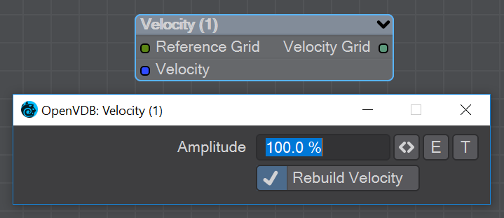
This node will construct a velocity grid for motion blur use.
- Reference Grid - Use to populate the velocity grid on the active values
- Velocity - Vector of velocity evaluated during grid building
- Rebuild Velocity - Rebuild Velocity at each evaluation rather than creating a static field
You can use an envelope or a texture map to adjust the velocity grid over time for more control
Visualize
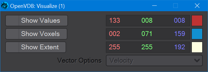
Additional Destination node to help visualize VDB networks. You can choose any combination of the three choices - Values, Voxels, and Extent. When this node uses a Velocity Grid output as its input, the Vector Options dropdown menu becomes available.
- Show Values - Shows the scalar voxel values multiplied by color
- Show Voxels - Show the voxel cubes
- Show Extent - Puts a box surrounding the voxel object showing the extents
- Vector Options - A dropdown menu with three options. This menu is ghosted when the Visualize node is not hooked to a Velocity Grid
- Velocity - Shows velocity unclamped transformed
- Normal - Shows normals scaled to .4 of box size to prevent overlap. Inverse transformed
- Color - Shows the color with no transform
OpenVDB Examples
- Example - First OpenVDB Liquid
- Example - Logo rezzing up
- Example - Volumetric Cheese
- Example - Chocolate Sauce Donut Drape