Node Editor

Click here to expand Table of Contents...

Introduction

This chapter is divided into two sections. First an overview of the Graphical User Interface (GUI) and some of the conventions used when working with nodes in the Node Editor. In the second section we will discuss each node individually and in detail in reference guide format for easy look-up of any node’s function, purpose and the various inputs and outputs associated with each.

The node editor is an alternative and superior way of shading and texturing the geometry created in the modeling process. Node-based editing systems such as commonly found in many high end 3D computer graphic applications, have established themselves as an industry standard tool for shading and texturing. The Node Editor in LightWave 3D is superior to many others combining the ease of use associated with LightWave 3D with the power and flexibility required by high-end industry professionals. As we will see, it is easy enough for a beginner to begin shading and texturing objects within just a few minutes and powerful enough for advanced users to design their own custom shaders and textures either by constructing special purpose node networks in the user workspace area or by using the LightWave 3D SDK that is offered free from NewTek Inc.

The Node Editor currently exists in three different places throughout the LightWave 3D working environment. Each environmental instance of the Node Editor is identical in operation and technique except for one key aspect - the Destination node, sometimes also referred to as the Root node.

There is always only one destination node for any attribute (volumetric lighting, vertex deformation, or shading and texturing) that nodes are applied to. Here are the three locations and an example of what each of the Destination nodes look like.

Displacement Destination Node

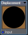
This will be the Destination node if the Node Editor is opened via the Edit Nodes button found in the Object Properties panel under the Deform tab (Accessed by pressing Shift-O, P).
Light Destination Node

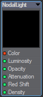
This Destination node will be present if the Node Editor is opened by clicking the Edit Nodes button located in the Volumetric Options panel contained in the Light Properties panel’s Basic tab (Accessed by pressing Shift-L, P).
Surface Destination Node

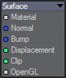
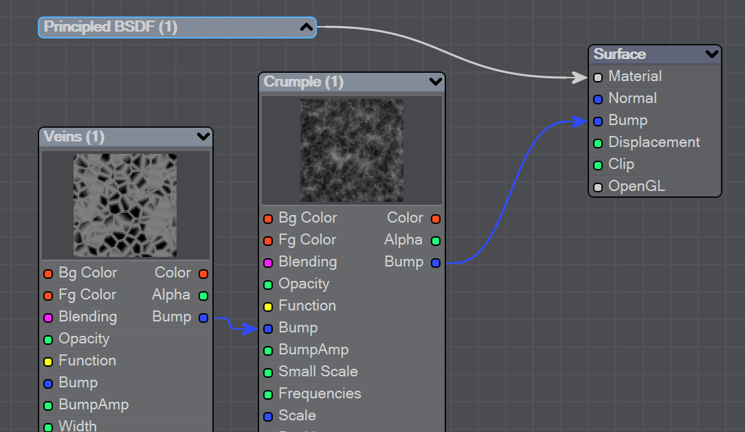
This is the Destination node you will be using if you open the Node Editor by clicking on the Edit Node Graph button found in the Surface Editor panel F5.

If you wish to mix bumps for separate materials into the surface, do not add them to the materials but directly into the destination Surface node as shown:

Input Node

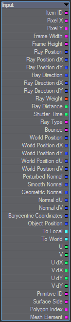
The Input Node is always present in a node editor, much like the Surface output node is in the Surface Editor’s Node Editor. It does not have to be used, but contains many frequently-required nodal inputs. There is an Input node in many of LightWave’s node editors, shown are Surface Editor, Nodal Motion, Nodal Texture, Nodal Displacement and Light Falloff. The Surface Editor Input node contains many new outputs:

Surface Input

When editing a surface, this node always appears in the Node Editor.

Item ID (Integer) - The LWItemID of the intersected primitive
Pixel X, Y (Integer) - The location of the pixel currently being rendered
Frame Width, Height (Integer) - The resolution of the image set in Camera Properties
Ray Position (Vector) - Origin of the ray that intersected this primitive (from the Camera, Reflection, Refraction, Shadow, etc.)
Ray Position dX, dY (Vector) - Ray origin differentials
Ray Direction (Vector) - The direction of the ray that intersected this primitive (from the Camera, Reflection, Refraction, Shadow, etc.)
Ray Direction dX, dY (Vector) - Ray direction differentials
Ray Weight (Color) The accumulated weight of the ray represented as a color
Ray Distance (Scalar) - The distance the ray traveled before intersecting the primitive
Shutter Time (Scalar) - The normalized shutter time (0...1)
Ray type (Integer) - Camera ray, Reflection ray, Refraction ray, Dissolve ray, Shadow ray and Occlusion ray. These can be fed into the Ray Type Switch node.
Ray Bounce (Integer) - The number of bounces the ray has taken to reach this intersection. Starts at 1
World Position (Vector) - The location of the intersection in world coordinates
World Position dX, dY (Vector) - The partial derivative of the world coordinate position in relation to X or Y coordinate of the pixel
World Position dU, dV (Vector) - The partial derivative of the world coordinate position in relation to the U or V coordinate of the pixel (for objects with automatic UV maps)
Perturbed Normal (Vector) - The interpolated normal perturbed by bump or normal mapping
Smooth Normal (Vector) - The interpolated normal
Geometric Normal (Vector) - The un-interpolated geometric normal
Normal dU, dV (Vector) - The partial derivatives of the normal along U and V coordinates
Barycentric Coordinates (Vector) - The masses of each vertex on a triangle
Object Position (Vector) - The location of the intersection in local coordinates
To Local, To World (Matrix) - Transformation matrices for the intersection
U, V (Scalar) - The U or V coordinate for the intersection, presuming the surface has UV coordinates
U and V dX, dY (Scalar) - The U and V partial derivatives along pixel X and Y
Primitive ID (Integer) - A Primitive can have an ID assigned that is different to the Item ID
Surface Side (Integer) - Determines if the intersection hit the front (0) or back (1) of the surface (2 double-sided back) (Example)
Polygon Index (Integer) - The numeric index for the polygon at the intersection
Mesh Element (Integer) - Outputs the element type needed for the Mesh Element Switch node

User Interface

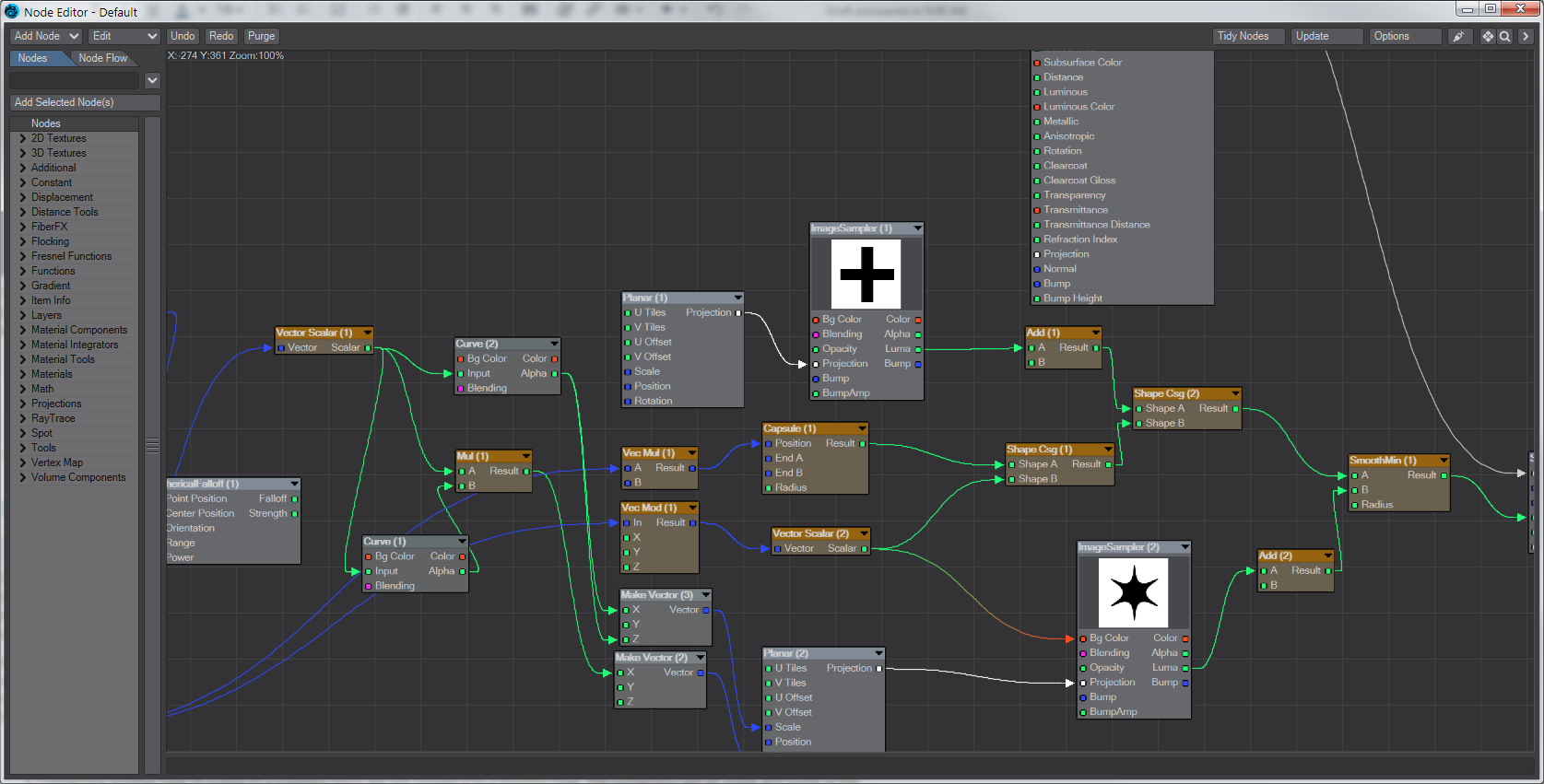
The Node Editor has improvements for LightWave 2019. The most obvious is the grid behind the nodes, but there are also improvements to the way the user interface works.

Grid

The grid display is constant and by default set to a size of 20 pixels. The shading of the grid is based on a difference from the background color of the Node Editor. The default is a difference of 8, but values can go as far as -128 to 128. Positive values will have a grid color lighter than the background, while a negative value will darken the grid in comparison with the background color. A value of 0 in the Grid Shade field will effectively hide the grid. Even invisible, the grid can still be snapped to and the top left corner of a node will be used as the snapping point.

Tidy Nodes

Rearranges nodes to remove overlaps. Tidy Nodes will also collapse nodes that are not in use and arrange all unused nodes in a column to the left of the network.

Keyboard Shortcuts

The LightWave standard of Ctrl+Alt will now zoom in and out of node networks to a minimum of 2 % and a maximum of 100 %. The zoom is based around the center of the network, similar to Layout zoom.

If you select a node, you can now tap the , (comma) key to select all the nodes upstream of the selected node, or tap the . (period) key to select all the nodes downstream. Nodes selected in this way will have thicker connection lines drawn.

You can now pan around the Node Editor space just using the MMB. There's no need to use Alt-LMB anymore, though you can continue to do so.

RMB Menu

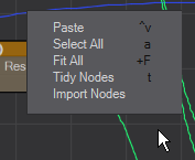
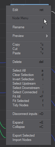
Left: nothing selected Right: one node selected

Clicking the Right Mouse Button (RMB) in the Node Editor will present one of two menus depending on whether you have node(s) selected or not. There are new entries in both menus for 2019.

Example - Getting Started with Nodes

Connection Types

There are eight kinds of connections in the Node Editor. Each type (listed below) is color-coded for your convenience. Color type connections are red, Scalar types are green, Vector types are blue, Integer types are purple, Functions are yellow, Projections are white, Transforms are cyan and finally Materials are light gray. Usually, you will want to keep the connections limited to only similar types but the Node Editor is very flexible and allows dissimilar types to be connected. This can be used to your advantage if you apply logic while constructing your networks.

It’s useful and sometimes necessary to mind which types you are connecting when creating a network. There are a few rules of behavior that you may count on from the Node Editor and like all rules there are a few exception to mind as well. One very advantageous rule is that when connecting dissimilar types the output type will be automatically converted to the input type that you are connecting it to, in the most intelligent way possible. There are only three exceptions to this and they are -

The Normal and Bump input in the destination Surface node prefer the incoming type to be a Vector , but you can equally add a Color or even a Scalar .
Connecting another type of output to a Function input will not convert it to a function type. The connection will be made and some of the information from the non-function output may be used but the results will be unpredictable. Functions are the only type of connection that are actually bidirectional. This bi-directionality is transparent to the user but Function nodes receive information from the node they are modifying, alter the information in some way and then send the results back to the node they are connecting to. A good general rule of thumb to remember about function-type nodes is just to not intermix them with dissimilar types. Keep your Functions in the yellow and all will be mellow.
Material inputs and outputs can only be attached to Materials .

Here is a matrix of the automatic conversion between same and dissimilar connection types of node inputs and outputs. It is repeated at the end of this chapter for quick reference.

Here is a description of the kinds of connections found in the Node Editor and some more of the rules that apply to each one in greater detail.

	To Color (Red)	To Integer (Magenta)	To Scalar (Green)	To Vector (Blue)	To Function (Yellow)	To Projection (White)	To Material (Gray)	To Extent (Dark Green)	To Volume (Dark Gray)	To Matrix (Cyan)
From Color (Red)	Color in RGB format unmodified	CCIR 601 Luminance values as Integer. Usually 0 or 1 only	CCIR 601Luminance values as float	RGB values copied to vector components respectively	N/A	N/A	N/A	N/A	N/A	N/A
From Integer (Magenta)	Integer value is duplicated to all 3 RGB channels	Integer value unmodified.	Integer value unmodified	Integer value copied to all 3 vector components	N/A	N/A	N/A	N/A	N/A	N/A
From Scalar (Green)	Scalar value copied to all 3 RGB channels	Rounded to the nearest Integer value	Scalar values unmodified.	Scalar value copied to all 3 vector components	N/A	N/A	N/A	N/A	N/A	N/A
From Vector (Blue)	Vector components are copied to RGB respectively	1st component ONLY is rounded to nearest Integer	1st component ONLY is used	Vector components unmodified	N/A	N/A	N/A	N/A	N/A	N/A
From Function (Yellow)	N/A	N/A	N/A	N/A	Receive, transform, return	N/A	N/A	N/A	N/A	N/A
From Projection (White)	N/A	N/A	N/A	N/A	N/A	Projection passed through	N/A	N/A	N/A	N/A
From Material (Gray)	N/A	N/A	N/A	N/A	N/A	N/A	Material properties passed	N/A	N/A	N/A
From Extent (Dark Green)	N/A	N/A	N/A	N/A	N/A	N/A	N/A	Extent values passed through	N/A	N/A
From Volume (Dark Gray)	N/A	N/A	N/A	N/A	N/A	N/A	N/A	N/A	Volume values passed through	N/A
From Matrix (Cyan)	N/A	N/A	N/A	N/A	N/A	N/A	N/A	N/A	N/A	Matrix values passed through

Color Type Connections

Color outputs and inputs are designated by a red dot next to the connection name. Color is a composite type connection containing three channels of information.

Input

Output

Color inputs receive incoming color connections as three channels red (R), green (G), and blue (B) from other nodes in the network you are currently working with. Most of the time you’ll want to connect colors to colors unless you have a very specific task in mind and have read this documentation thoroughly fully understanding the consequences and conversions that take place when making connections between dissimilar connection types.

Connecting non-color output from other nodes to a Color input will automatically copy the incoming values to each color channel red, green, and blue. The color of the line connecting the two dissimilar types will change over the lines length from whatever color designates the output selected to red.

If the incoming connection is a vector type output then XYZ or HPB etc., will supply the values for the RGB respectively. This means that if the incoming vector type is a Position for example, then the X value of that vector will be used to define the red channel of the color. Y to green, and Z to blue and so on in a similar way for HPB if the vector being used is a rotation and so on.

The vast majority (almost all) of connections in the Node Editor are evaluated per spot therefore if the incoming color connection has a variance in the shader or texture values that is affecting the color channel (i.e. a pattern of some kind) then that varied color value will be supplied to the color input it is connecting to. Simply put, if you connect the color output of a red and green marble texture to a color input then that input will receive a red and green colored marble pattern - evaluated on a spot by spot basis.

Color outputs always supply three channel data evaluated per spot, in the format red, green, and blue (RGB) regardless of what other inputs are connected to the node or what other settings you may have set for your scene. Even if the incoming data for the node’s colors are scalar values and/or you have selected gray values via the color picker panel, the color output will still be outputting three channels of data.

Scalar Type Connections

Scalar outputs and inputs are designated by a green dot next to the connection name. In LightWave 3D’s Node Editor, a scalar is a floating point number or quantity usually characterized by a single value which doesn’t involve the concept of direction. The term scalar is used in contrast to entities that are “composites” of many values, like vector (XYZ, HPB, etc.), color (RGB), etc.

Some examples of scalar values are: 3.14159265, 13, 0.00001, -5.5, 2, and 69.666

Input

Output

Primarily, connections to a scalar input will be scalar outputs from other nodes in the network you’re working with. Most of the time you’ll want to connect scalars to scalars unless you have a very specific task in mind and have read this documentation thoroughly fully understanding the consequences and conversions that take place when making dissimilar connections.

Connecting non-scalar output values to a scalar input will automatically convert it to scalar type. The color of the line connecting the two dissimilar types will change over the lines length from whatever color designates the output selected to green.

If a component (vector or color) type output is being connected to the scalar input then one of several things may happen as follows:

If it is a color type output that is being connected to the scalar input then the CCIR 601 luminance values for that color are derived from the RGB values and used as the scalar input.

If it is a vector type output that is being connected to the scalar input then only the first component of the vector is used as the scalar value. For example if the vector being used is a position then only X will be supplied to the scalar input and Y and Z will be ignored. Likewise if the vector being used is a rotation then only the H (heading) will be used and the P (pitch) and B (bank) channels will be ignored.

Again however, these conversion processes are automatic and transparent to the user.

Scalar outputs from any given node will always supply scalar values regardless of what other inputs are connected to the node. Please see above for examples of scalar values.

Integer Type Connections

Integer outputs and inputs are designated by a purple dot next to the connection name.

Integers in the Node Editor can be used for many things but most often they are designated for the purpose of specifying predefined list member items such as any of the Blending modes described below in the next section on Blending Modes (see the Blending Modes table further down).

An integer is a non-floating point natural number. Some examples of integers are: 3, 13, 0, -5, 69 and 666.

Input

Output

Primarily connections to an integer input will be integer outputs from other nodes in the network you’re working with. Most of the time you’ll want to connect integers to integers unless you have a very specific task in mind and have read this documentation thoroughly thus fully understanding the consequences and conversions that take place when making dissimilar connections.

Connecting non-integer outputs to an integer input will automatically convert it to integer type using standard rounding. The color of the line connecting the two dissimilar types will change over the lines length from whatever color designates the output selected to purple.

If a component type output is being connected to the integer input then one of several things may happen as follows:

If it is a color type output that is being connected to the integer input then the CCIR 601 luminance values for that color are derived from the RGB values. Those luminance values are then rounded and used as the integer input. Since internal luminance values in the Node Editor are floating point values which most often range from 0.0 (black) to 1.0 (white) the rounding that takes place during this conversion would have the effect of reducing the luminance information to either a value of zero or one with no gray tones in between. Consider that the luminance value 0.5 (50% gray) when rounded to an integer value would become a value of 1 (white) and a gray tone just slightly below 50% gray (0.4) when rounded to an integer value would be 0 (black).

If it is a vector type output that is being connected to the integer input then only the first component of the vector is used after rounding it, as the integer value. For example if the vector being used is a rotation then only the rounded H (heading) value will be supplied as the integer input and P (pitch) and B (bank) will be ignored. Likewise if the vector being used is a scale or position then only the rounded X value will be used and the Y and Z channels will be ignored.

These conversion processes however, are automatic and transparent to the user.

Integer outputs from any given node will always supply integer values regardless of what other inputs are connected to the node. Please see above for examples of integer values.

Vector Type Connections

Vector inputs and outputs are designated by a blue dot next to the connection name.

Vectors are composite type values meaning they are comprised of more than one component or “channel”. Some examples of vectors in the Node Editor are Position, Scale, and Rotation. Notice that each one of these attributes contain more than one value. For example position is comprised of X, Y and Z. Scale is also comprised of X, Y, and Z and rotation is comprised of H, P and B - Heading, Pitch, and Bank respectively.

Input

Output

Generally, connections to vector type inputs will be vector type outputs from other nodes in the network you’re working with. Most of the time you’ll want to connect vectors to vectors unless you have a very specific task in mind and have read this documentation thoroughly thus fully understanding the consequences and conversions that take place when making dissimilar connections. You will never want to connect anything other than a vector type output to a vector type input that is labeled “Normal” next to the blue dot designation unless you know ahead of time why. The case for needing to make such kinds of connections to a Normal input is so rare that in fact the destination Surface node disallows non-vector connections to it’s Bump and Normal vector inputs. The general rule of thumb here is that all Normal inputs should only be receiving their data from other Normal type outputs. You may remember it by learning: “Normals in like only Normals out.” where the inverse of that phrase may not always be true.

Connecting non-vector output types to a vector input will automatically convert it to vector type with various limitations. The connection will be made except where noted, and the color of the line connecting the two dissimilar types will change over the lines length from whatever color designates the output selected, to blue.

Color type outputs are a kind of vector although undesignated as such and for good reason. It can be quite confusing to discuss colors as vectors. However there are times when the relationships are straightforward enough to be immediately useful.

When connecting a color output to a vector input each channel of the color output (R, G, and B) will be used to define the first, second, and third components of the vector respectively.

If a non-component type (scalar or integer) output is being connected to the vector input then the value of the scalar or integer is copied into all of the components of the vector that it is being connected to. For example connecting an Alpha output from any of the texture nodes to any of the texture nodes input connections labeled Scale would copy the Alpha value to all three of the components of the Scale vector. If for example, the Alpha value was 1.0 the recipient textures Scale value would be 1.0 for X, Y, and Z.

Once again these conversion processes are automatic and transparent to the user.

Vector outputs from any given node will always supply vector component values regardless of what other inputs are connected to the node.

Function Type Connections

Function type connections are special two-way connections. Functions offer a way of transforming a texture or shader value based on the functions’ graph.

Input

Output

Function inputs should only be connected to from other Function type nodes in the network you are working with.

Always connect function to functions.

Connecting non-function outputs to Function inputs will make the connection and the color of the line connecting the two dissimilar types will change over the lines length from whatever color designates the output selected, to yellow. However the results of dissimilar connections with function nodes are not guaranteed to produce any predictable results.

When a function output is connected to a function input data (usually texture value data) from the node being connected to is sent to the connecting node where it is then transformed and sent back to the recipient node. The transformations that occur depend entirely upon the kind of Function node that is being used and the settings entered for its graph.

Function nodes specifically utilize the function connection to transform values of the nodes they are connecting to. Typically this will be shaders and textures and in these cases the shader or texture sends the shader or texture value to the connected function node. The connected function node then transforms these values based of the function graph, and returns the transformed values to the recipient node.

Function connections are specialized in this way allowing for bidirectional communication between nodes.

Once again, the output of a Function type connection should always be connected to the input of another Function type connection.

Material Type Connections

Material inputs and outputs are designated by a light gray dot next to the connection name.

Where previous connections were for input specific channels into other nodes, Materials are complete in themselves.

Input	Output
Can only be connected to by other Material outputs	Can only be connected to other Material inputs

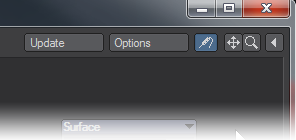
Node Editor Probe

Item #8 in the initial guide to the Node Editor, this is a node probe that will show you the outputs of the nodes in your network.

When enabled, you can hover the mouse cursor over any node’s output connections or preview area. If the preview area has a standard preview sphere, the hover location is displayed in the preview data type (color, scalar, vector, integer, etc.) When hovering over an output connection, the displayed data uses the data type of that connection; however, the value is evaluated without the knowledge of any ray trace environment. Therefore, the output connection evaluation is really only useful for those nodes that do not use preview spheres. The data display is shown in a floating popup that follows the mouse.

The data display will update a few times per second to account for live input from a Device node or if the user updates the preview spheres manually via the space bar. In other words, the mouse pointer can continue to hover over the same screen position and whatever happens to be beneath it will be displayed automatically.

The preview sphere has traditionally been a gamma-corrected appearance of the actual evaluation. The probe will display the source data for the preview sphere, not the altered visual representation. The probe then shows the value of that output not the color-adjusted grayscale representation of that value.

Blending Modes

Value	Blending Mode
0	Normal
1	Additive
2	Subtractive
3	Multiply
4	Screen
5	Darken
6	Lighten
7	Difference
8	Negative
9	Color Dodge
10	Color Burn
11	Red
12	Green
13	Blue

All of the blending modes in the Node Editor are based on their Photoshop equivalents. Here is a description of each one not defined elsewhere in the LightWave 3D manual:

Darken

Darken looks at the foreground and background colors and chooses the darker one, whichever it is. Whichever is darker wins. Which of the two is used will vary across the image depending on which is darker at each spot as it is evaluated.

Lighten

Lighten is the reverse of darken. It evaluates the foreground and background colors and replaces the darker ones with the lighter ones.

Color Dodge

Color Dodge is a kind of inverted multiply mode. Dodging is a dark room technique commonly used by photographers and photo developers. This analog equivalent technique is achieved by holding a small piece of cut paper taped to the end of a thin wire or stick, in between the projected light and the photo paper causing some areas of the photograph to be underexposed. The same thing is going on here but the foreground pattern is being used as the dodge mask instead of a cut to shape piece of paper, to underexpose those areas. Remember that the more underexposed an area is the lighter it is and a completely unexposed sheet of photo paper is all white.

Color Burn

Color Burn is basically the same thing in reverse. Burning is also a darkroom technique where (in its simplest form) a large piece of paper with holes cut in the middle is held between the projected light and the photo paper after exposing the image initially on to the paper. This has the effect of overexposing or burning in some areas of the image. Again it is the background color values and patterns that are being used in place of that cut sheet of paper just mentioned, to burn in the image. Remember that the more overexposed an area is the darker it is and a completely overexposed sheet of photo paper is all black.

Red

Colors as seen on your monitor are comprised of three components red, green and blue. Each of these primary colors can be talked about or represented by considering them as separate channels. Usually to form any specific color these three channels are mixed additivly.

In these next three blending modes we are able to use each unique channel individually.

Selecting Red as the blending mode replaces the blue and green of the FG color channels with the blue and green channels contained in the BG Color. Only the foreground’s red channel will be considered but the green and blue channels will be taken from the background color only. If for example, your background color was 100% blue and your foreground color was 100% red - selecting Red as the blending mode would result in purple output.

Green

Selecting Green as the blending mode replaces the blue and red channels of the FG color with the blue and red channels from the BG Color. Only the foreground’s green channel will be considered but the red and blue channels will be taken from the background color only.

Blue

Selecting Blue as the blending mode replaces the red and green channels of the FG color with the red and green channels contained in the BG Color. Only the foreground’s blue channel will be considered but the red and green channels will be taken from the background color only.

Opacity

Opacity is the amount that each of these blending modes mentioned above, is applied. You can think of opacity as the strength of the blend effect.

Invert

The Invert toggle button inverts the scalar Alpha values used to blend the two colors; background and foreground. Where applicable it will also invert the bump gradient so that not only are the background and foreground colors are swapped but the bump and alpha outputs as well are inserted.

About Using Nodes

All the nodes and textures included in LightWave 3D are multipurpose. Some textures are useful for things that you would not immediately recognize them as being useful for. For example, Bricks2D can be used to make strange-looking spider webs and a various assortment of other similar patterns.

It’s good practice to work with VPR (Ctrl -F9) active at all times while creating networks with the Node Editor. It is also very beneficial to have the Surface Presets shelf (F8) open during any surfacing work. VPR and the Presets shelf work together to offer the user a convenient interactive work history during the process of constructing texturing or shading Networks. Double clicking on the preview display area in the Surface Editor will add an entry in the Presets shelf with a scale version of that image as the icon for that preset.

Conversely, double-clicking on an icon in the Presets shelf will load and apply all of the surface settings saved when you double clicked on the Surface Editor preview display area.

Common Inputs and Outputs

Rather than repeating the same information all the time it makes more sense to only detail unique Inputs and Outputs and refer to a single place for the documentation of items shared between nodes. Herewith the Inputs and Outputs common to all nodes, starting with Inputs:

Inputs

Bg Color (Color) - Can receive colors and patterns from other nodes in the network. Users may also specify a background color using the controls found in the Edit Panel for this node.
Fg Color (Color) - Can receive colors and patterns from other nodes in the network. Users may also specify a foreground color using the controls found in the Edit Panel for this node.
Blending (Integer) - Specifies one of the blending types (0~13) found in the blending type list at the beginning of this chapter.

Can receive input from other nodes in the network or can be specified to by selecting a blending mode from the Blending pull-down menu in the Edit Panel for the node.

For general use specifying the blending mode by using the Blending pull-down menu in the Edit Panel will probably be the most desirable method of use. However, for larger networks where control of the blending modes of many texture nodes simultaneously is needed or when conditional blending is desired then using a node connection to control this value may be advantageous.

Opacity (Scalar) - Opacity is the amount that the selected blending mode is applied. You can think of opacity as the strength of the blend effect between the BG Color and the FG Color.

Can receive patterns and numerical inputs from other nodes in the network. The user may also specify this parameter value using the controls available in the Edit Panel for this node.
U Tiles (Integer) - Specifies the number of tiles in the U dimension.

Can receive patterns and numerical inputs from other nodes in the network The user may also specify this parameter value using the controls available in the Edit Panel for this node.
V Tiles (Integer) - Specifies the number of tiles in the V dimension .

Can receive patterns and numerical inputs from other nodes in the network The user may also specify this parameter value using the controls available in the Edit Panel for this node.

Fractal Inputs

Small Scale (Scalar) - Like Lacunarity, Small Scale is a counterpart to the fractal dimension that describes the texture of a fractal. It has to do with the size distribution of the gaps between detail levels. The Small Scale value sets the amount of change in scale between successive levels of detail.

If you are seeing repeating patterns in the texture it might be a good idea to alter the Small Scale value for the texture.

Can receive patterns and numerical inputs from other nodes in the network. The user may also specify values for this attribute using the controls available in the Edit Panel for this node.
Contrast (Scalar) - Sets the contrast of the texture value gradient. Higher values produce less gradient information between texture value extremes and therefore less noise is produced. The lower values spread the gradient more evenly between the extremes of the texture values and thus allow for more overall noise in the final output from this node.

Can receive patterns and numerical inputs from other nodes in the network. The user may also specify the values for this attribute using the controls available in the Edit Panel for this node.
Frequencies (Scalar) - “Frequencies” as used in this node is really just another name for octaves as defined in some of the descriptions of fractal type textures within this document.

You can think of “Frequencies” as the number of levels of detail mentioned in the discussion just above for Small Scale. At one “Frequency”, only the basic pattern is used. At 2 “Frequencies” given a Small Scale value of 2, a one half scale pattern is overlaid on top of the basic pattern. And at three Frequencies, the overlays are one quarter scale over the one half scale over the basic and so on.

If Small Scale were 3 in this example, it would mean that each new iteration would be one third the scale of the previous layer.

Can receive patterns and numerical inputs from other nodes in the network. The user may also specify the values for this attribute using the controls available in the Edit Panel for this node.
Increment (Scalar) - Since this texture is a fractal or a fractalized noise pattern, it means that we can overlay smaller and smaller copies of the same pattern functions over previous layers in order to add detail. Technically, this is called Spectral Synthesis. These are not surface layers, but layers considered within the algorithm of the texture node itself.

Increment is the amplitude or intensity between successive levels of detail.

Can receive patterns and numerical inputs from other nodes in the network. The user may also specify this parameter value using the controls available in the Edit Panel for this node.
Lacunarity (Scalar) - Lacunarity is a counterpart to the fractal dimension that describes the texture of a fractal. It has to do with the size distribution of the holes. Roughly speaking, if a fractal has large gaps or holes, it has high lacunarity; on the other hand, if a fractal is almost translationally invariant, it has low lacunarity. The lacunarity value sets the amount of change in scale between successive levels of detail.

If you’re seeing repeating patterns in the texture it might be a good idea to lower the lacunarity level of the texture.

Can receive patterns and numerical inputs from other nodes in the network. The user may also specify this parameter value using the controls available in the Edit Panel for this node.
Octaves (Scalar) - You can think of octaves as the number of levels of detail mentioned in the discussion just above for lacunarity. At one octave, only the basic pattern is used. At 2 octaves given a Lacunarity value of 2, a one half scale noise pattern is overlaid on top of the basic pattern. And at three octaves, the overlays are one quarter scale over the one half scale over the basic and so on.

If Lacunarity were 3 in this example, it would mean that each new layer would one third the scale of the previous layer.

Considering these three Increment, Lacunarity, and Octaves then if Lacunarity were set to 2, Increment were set to 0.5, and Octaves were 4, it would mean that each successive iteration for 4 iterations, was twice the frequency and half the amplitude.

Can receive patterns and numerical inputs from other nodes in the network. The user may also specify this parameter value using the controls available in the Edit Panel for this node.
Offset (Scalar) - Defines an offset into the texture value range where the minute details produced by the combined effects of Lacunarity, Increment, and the number of Octaves, begin to ramp sharply.

Can receive patterns and numerical inputs from other nodes in the network. The user may also specify this parameter value using the controls available in the Edit Panel for this node.

Function Inputs

Frequency (Scalar) - The Frequency input controls the time taken to complete one function cycle. By increasing the frequency, the cycle period of the function is reduced. Likewise, decreasing the frequency means the function takes longer to complete one whole cycle. The mode (described below) determines the behavior of the function once it has completed a full cycle.
Amplitude (Scalar) - The Amplitude input controls the size of the function from peak to peak.
Phase (Scalar) - The Phase input allows the function waveform to be shifted in time. Increasing the phase shifts the function to the left, while decreasing it shifts the function to the right.
Mode (Constant, Repeat or Oscillate) - Three modes are available that determine how the function behaves after one complete cycle has been performed. The possible choices are:

Constant mode - in which the function remains as its last value when one cycle completes.
Repeat mode - in which the function restarts from the beginning when one cycle completes, giving a repeating oscillation based on a saw tooth waveform.
Oscillate mode - in which the function completes one cycle and then returns to its start point over the next cycle. This provides a repeating oscillation based on a triangular waveform.

Clamp Low (Scalar) - The Clamp Low input defines a point at which, if the function is less than, the output is clipped. In other words the output of the function can be no lower than this value.
Clamp High (Scalar) - The Clamp High input defines a point at which, if the function is greater then, the output is clipped. In other words the output of the function can be no higher than this value.
Begin (Scalar) - The Begin input specifies the start of the step. That is, the position for the start point of the ramp up.
End (Scalar) - The End input specifies the finish of the step. That is, the position for the end point of the ramp up.

Material Inputs

Specular/Specularity (Scalar) - The term specular or specularity here refers to the optical property referred to in previous LightWave surface terms as reflection. The difference with standard Surface Editor Reflection where you can have as much as you like while also keeping the Diffuse level high, in a Material raising one will lower the other keeping the balance physically correct between the two.
Roughness (Scalar) - This value does nothing on its own. It is designed to be used with Reflection and Refraction Blur on the Advanced tab. Likewise, without some degree of Roughness , those settings do nothing except slow the render slightly.
Absorption (Scalar) - How quickly light passing inside an object is extinguished. A low value here with indicate greater transparency. Based on Beer’s law of absorption, to give a more realistic and non-linear result.
Refraction Index (Scalar) - This value is for the Index of Refraction of your material. Often used - 1.33 for water, 1.5 for glass, 2.4 for diamond.
Dispersion (Scalar) - Controls the amount of light dispersion. Dispersion is a phenomenon that causes the separation of a wave into spectral components with different wavelengths, due to a dependence of the wave’s speed on its wavelength. This will cause the surface to render more slowly as it renders each spectral component separately (red, green and blue).

Dispersion as used in this shading model simulates real light dispersion. The higher the value the greater the amount of dispersion that will be simulated and applied.
Normal (Vector) - Specifies a vector direction for modifying the surface normal and only Tangent Normal maps should be used. This is surface normal direction information and affects the way the surface is shaded. Care should be taken when connecting to this input. Connecting dissimilar types or non directional vectors may cause the surface to shade wrongly.
Bump (Vector) - Specifies a vector direction for modifying the surface bump. This is surface normal direction information and affects the way the surface is shaded. Care should be taken when connecting to this input. Connecting dissimilar types or non directional vectors may cause the surface to shade wrongly.
Bump Height (Scalar) - Specifies the bump height or “amplitude” of the Bump directional vectors.
Bump Dropoff (Scalar) - How fast the visibility of the bump falls away.

Material Advanced Inputs

The Advanced tab contains controls common to all Materials namely Reflection and/or Refraction Blurring and environment settings similar to the standard Surface Editor’s Environment tab.

Reflection Blur - Controls the amount of blur of the surface reflections. Some amount of blur is required in order to have the Dispersion amount (when available) affect the surface.
Mode / Reflection Image Mode and Image are features exclusive to the Edit Panel. Please see the explanation for these items in the chapter that covers texturing with the Surface Editor.
Image Seam Angle - allows the user to rotate the seam line of a wrapped image around the Axis that has been selected for the projection method.
Interpolated - Switch between standard unified sampling and using a defined Sample and Blend Size to tailor your surface.

Outputs

Color (Color) - Outputs three channel color information in R, G, B format, evaluated on a per spot basis.
Alpha (Scalar) - Outputs single channel alpha (grey) information evaluated on a per spot basis.
Luma (Scalar) - Outputs CCIR 601 luminance values derived from the RGB values contained in the image being used.
Bump (Vector) - Outputs component vector direction information the length of which are the product of the bump amplitude value.
Normal (Vector) - Outputs component vector direction information the length of which are the product of the bump amplitude value.

If used as an input to another normal type connection the destinations normal will be completely replaced with this information.

Nearly all Inputs can receive patterns and numerical inputs from other nodes in the network. The user may also specify this parameter value using the controls available in the Edit Panel for this node.

Edit Panel

Radiosity and Caustics check boxes are not offered as node connections in the Workspace area and are features exclusive to the Edit Panel of the node.When checked this shading model will evaluate shading information for the surface channel it is being applied including any Radiosity or Caustics computations as defined by those system attributes applied to the scene.

Unchecked, radiosity and/or caustics calculations will not be evaluated by this shading model as it is applied to the object surface being edited.

This can be used to omit both entire surfaces or per channel surface attributes from radiosity or caustics calculations thus offering more diversity in the rendered output as well as reducing the time needed to calculate these surfaces in scenes where either radiosity or caustics are used.

Noise Type

You can get a very good idea of what each Noise Type looks like in the fractal-based Node edit panel by following these few simple steps:

Set the texture Scale values small enough that you can see the full pattern of the texture on the geometry you’re working with.
Set Increment to zero.
Set Lacunarity to zero.
Set Octaves to zero.
Set the Offset value anywhere between 0.25 and 0.75
And select the various Noise Types one at a time while watching the VPR preview update.